SeqGeq Basic Tutorial (SeqGeq v1.6.0)
This tutorial is designed to give researchers a basic overview of the features and functions available in the SeqGeq bioinformatics analysis platform.
All data files illustrated here are available as demo data included in the installation of SeqGeq. Specifically, analyses illustrated here will focus on the 6K_PBMC.csv data file.
*Analysis performed in this tutorial should be considered as demonstration of features only. Researchers are encouraged to independently vet and validate their own workflows as much as possible.
Table of Contents:
1 – Install
2 – Logging In
3 – The Workspace
4 – Loading Data
4.1 – Populations
4.2 – Genesets
5 – Gating
5.1 – Cell View
5.2 – Gene View
6 – Quality Control
6.1 – Quality Cells 17
6.2 – Quality Genes 18
7 – Dimensionality Reduction 20
7.1 – PCA 20
7.2 – tSNE 24
8 – Clustering 26
9.1 – Setup
9.2 – Volcano Plots
10 – Geneset Enrichment
10.1 – Geneset Libraries
10.2 – Running Geneset Enrichment
11 – Exports
11.1 – Populations
11.2 – Statistics
11.3 – Genesets
11.4 – Figures
11.5 – Workspaces
12 – Plugins
12.1 – Setup
12.2 – Running
12.3 – Developers
12.4 – Highlights
13 – Resources
13.1 – Educational
13.2 – Research Tools
13.3 – Bioinformatics Platforms
13.4 – Help
1. Install
Installers for SeqGeq are available from the Downloads tab of the SeqGeq solutions section of the FlowJo.com website:
flowjo.com/solutions/seqgeq/downloads
Installers are offered for both Mac (OSX 10.8+) and 64bit Windows operating systems. After downloading the appropriate installer for your system, simply run that EXE or DMG file, and follow the instructions given, in order to put the SeqGeq software platform onto your machine.
Note: SeqGeq is not supported on 32bit Windows machines.
2. Logging In
Logging into SeqGeq requires that a researcher create an account in the FlowJo Portal environment, and an activated SeqGeq license there. To sign up for, and activate a free FlowJo Portal account, visit the following site:
Users can get an active license to try SeqGeq Free by signing up for a trial account within the FlowJo Portal:

When running SeqGeq you’ll be prompted to enter your FlowJo Portal credentials:

Note: Clicking Demo there will open SeqGeq in demo mode, where only the demo data which comes with the SeqGeq install can be loaded.
3. The Workspace
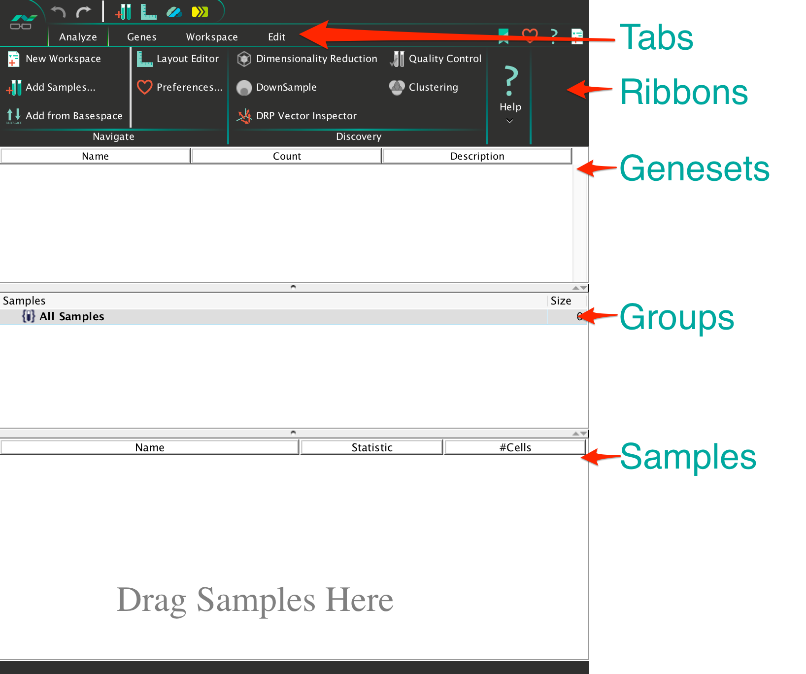
SeqGeq’s Workspace contains some general areas such as Tabs, Ribbons, Genesets, Groups and Samples.
- Tabs contain Ribbons with various features, grouped by common functions:
- The Genesets area of the workspace will contain sets of parameters as they are either loaded from CSV files into SeqGeq, or defined within SeqGeq based on data analyzed there.
- Groups will separate out different samples from the All Samples group, and can contain gates or statistics just like an individual sample.
- The Samples area of the workspace will illustrate samples within the group selected. Those samples will contain hierarchically ordered nodes representing the analysis performed on them. This can include nodes representing: Plugins, Statistics, Populations, Gates, or any other platforms in SeqGeq.
Ribbons within the tabs of the workspace can be customized to contain sections according to your prefered organization, by clicking on the Customize Ribbon icon in the top right hand corner of SeqGeq’s workspace and dragging options from there into the ribbons area of a tab. Try adding the Boolean ribbon to the Workspace tab of your workspace:

Saving, opening and quitting a workspace can be accomplished by clicking on the SeqGeq button in the top left hand corner of the workspace:

4. Loading Data
Dragging and dropping data into the SeqGeq workspace will load that data within the platform. Within the Analyze tab there’s a Navigate option, which also contains functions for loading data from your file system, or directly from Illumina’s BaseSpace application:

Another type of data which can be dragged into the SeqGeq workspace consist of CSV lists of genes (aka Genesets).
Note: SeqGeq has been designed to accept data from all sequencing pipelines. In other words we try very hard to be “data agnostic”. If you’re finding data that SeqGeq won’t load we encourage you to submit a demo data-set to seqgeq@flowjo.com for further investigation and troubleshooting.
4.1 Populations
Populations are simply data matrices containing cells (aka events) within SeqGeq. These samples can then be subdivided into sub-populations using gates within the Cell View of a Graph Window corresponding to that sample.

4.2 Genesets
Genesets are groups of parameters within SeqGeq. These lists of parameters can be organized into Collections for the sake of convenience and clarity:

Double-clicking on a Geneset will open a geneset inspector where you can investigate the genes comprising that Geneset:

5. Gating
Gating tools are available at the top of SeqGeq’s Graph Window which can be opened by double-clicking on any population within the workspace. Within the resulting display, users will be able to search the parameters (genes / antibodies / categoricals / derived parameters) available within their data set. This search function is enabled by an x-wing and y-wing for each axis within the Graph Window:

Gating is a fundamental feature within SeqGeq with which many different workflows are built. Gates can be developed hierarchically such that each new gate is built upon a foundation of other gates created upstream. Often this gating tree leads to a complex and nuanced data analysis leading to important research and entirely novel discovery.
5.1 Cell View
Gating in the Cell View of SeqGeq’s Graph Window filters cells into subpopulations. Where parameters are available from upstream data collection and have been merged with the transcriptomics (gene expression matrix), such as flow cytometry or imaging cytometry, these gates can be particularly useful:

Parameters available for gating in Cell View will depend on the parameters present in a given expression matrix loaded there. Parameters combined into Genesets will also perform as parameters themselves, whose values rely on a summary statistic (such as ‘Median’) of the genes within that Geneset:

The Cell View Graph Window also gives researchers the feature to color map dots using a tertiary parameter. This can be very useful for illustrating the values of a categorical parameter, or the expression of a specific gene of interest within dimensionally reduced space:

5.2 Gene View
Clicking on the “Gene View” button at the top of SeqGeq’s Graph Window will change the plot from Cell View to Gene View. In Gene View parameters (genes, antibodies, categoricals and/or derived parameters) are displayed as dots, rather than cells. This means that the axes within the Gene View are populations, and the value displayed for each parameter (dot) will be that gene’s mean expression with regard to x and y populations.
Gates drawn in Gene View will not create populations, but will rather produce a Geneset at the top of SeqGeq’s workspace, grouping parameters contained in the geometry of the gate drawn within that Geneset:

Note: All Genes are displayed in the Gene View by default, but users can select the Geneset to view there within the top left hand corner of that Graph Window.
6. Quality Control
The first step in analyzing data will typically be to perform some quality control. Clicking the “Quality Control” button within SeqGeq will open up three graph windows. One in Cell View and two in Gene View. The parameters illustrated there are only created once that button is clicked, and contain derived information calculated for each cell and each gene. We call these parameters Derived Parameters (DPs) and Derived Observations of Genes (DOGs) respectively.

Note: The quality control process can be repeated for subpopulations of interest within a sample, as the genes of interest for the raw data may not be appropriate, or important relative to deeper populations of cells.
6.1 Quality Cells
Quality control on cells removes outlier events which might represent empty wells, or doublets based on the cell’s Library Size versus the number of Genes Expressed:

6.2 Quality Genes
Researchers may also want to perform quality control on their genes to isolate those most conducive to good clustering and the best possible population separation in dimensionality reduction.
The first Gene View for Quality Control illustrates Total Expression for every gene, versus the # of Cells Expressing each gene. Though this set of parameters are linear by default, try changing the transform applied to them by clicking the “T” buttons next to both axes and utilizing the Log axis option there, and gate to remove dimly expressed genes and genes expressed in most cells (housekeeping):

Note: The options in the “T” (for ‘Transform’) button there can be applied to any parameters in any Graph Window within SeqGeq to change scaling. The Customize Axis options there can give particularly great control over the view of parameters analyzed.
The second Gene View graph that’s displayed from the Quality Control button is with regard to Cells Expressing each gene and Dispersion. Dispersion is related to variance, and variance tends to correlate with the ability of a parameter to separate biologically relevant populations within data matrices. Therefore researchers may want to select for highly dispersed genes.
Try viewing the genes identified from the first Quality Control Gene View within this second Gene View Graph Window, and gate highly dispersed genes within that Geneset:

Note: When available External RNA Consortium Controls (ERCCs) can be used to gauge the cut-off for high dispersion.
7. Dimensionality Reduction
Dimensionality reduction is an invaluable tool for analyzing high parameter data-sets. In various ways it allows researchers to visualize high dimensional data within a smaller number of parameters while maintaining a high degree of variability and separation between distinct cell populations.
7.1 PCA
The simplest form of dimensionality reduction available in SeqGeq is the machine learning algorithm for Principal Component Analysis (PCA). This is also typically the first dimensionality reduction technique applied to a sparse data-set for further downstream analysis after quality control.
To run PCA, select a population of interest, click on the Dimensionality Reduction button within the Analyze tab in SeqGeq’s workspace, and choose PCA:

Within that dialog you’ll likely want to normalized selected genes, log transform the parameters (to maximize the dynamic range available for separation of populations), and you’ll need to choose the genes on which you’d like to base your principal components computed.
The platform will display a table of variance described by each of the principal components. Principal components selected there will be added as parameters to your data as “Analytical Parameters”:

Try running PCA on the quality cells population using your highly dispersed genes Geneset:

Note: Islands illustrated in this visualization represent broadly distinct neighborhoods of populations within the data matrix.
7.2 tSNE
The tSNE machine learning algorithm is a much more advanced tool for non-linear dimensionality reduction. Our implementation reduces a data matrix input to just two parameters, tSNE X and tSNE Y. This technique is widely used in visualizations across multiple disciplines, because it has the ability to describe a high amount of local variability among populations out of N-dimensional space, while projecting into a simple and easy to understand 2-3 dimensions.
To run the tSNE visualization select a population of interest, (re-) engage the Dimensionality Reduction button within the Analyze tab in SeqGeq, choose the “tSNE” option there, and select the parameters or genes you’d like to input (map into two dimensions). Typically principal component parameters are used to map single-cell RNA sequenced data with tSNE, as these represent a more rich (less sparse) interpretation of the data.
Within the tSNE section of the dimensionality reduction platform there are a number of settings, including Advanced Settings which can be used to adjust the tSNE algorithm calculations. Mousing over these different options will give feedback regarding the function of each:

Try mapping your principal components developed from the highly dispersed genes into tSNE space – If you normalized genes for your PCA, you won’t need to normalize those parameters in tSNE:

8. Clustering
SeqGeq currently (v1.4.0) offers K-Means clustering within the Clustering platform. K-Means is a machine learning algorithm that places events into one of ‘k’ unbiased clusters, where ‘k’ is an integer set by the researcher.
To run the K-Means clustering, select a population of interest within the workspace, and click on the Clustering button within the Analyze tab of the workspace. In the resulting dialog select the parameter on which you want the clustering to run, and choose your desired k number of clusters to calculate:

K-Means will generate a new parameter which separates clusters by integer values. In order to automatically gate these cluster values into populations, its very useful to take advantage of the AutoGateCategorical plugin, which comes installed by default in SeqGeq. To access and run this plugin, simply select your population of interest, navigate to the Workspace tab of the workspace, and select AutoGateCategorical from the Plugins dropdown list there:

Within the plugin dialog select the K-Means parameter and run the plugin:

This will generate populations corresponding to clusters defined by K-Means:

Try running K-Means clustering on your Quality Cells population, using the principal component parameters calculated previously, and color map those clusters onto your tSNE parameters:
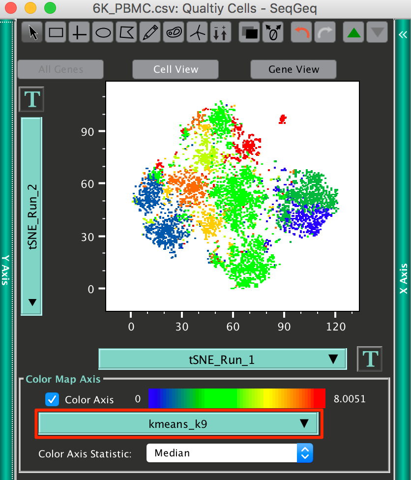
Note: Each color within the color mapping here represents one of the K-Means clusters within the data.
9. Differential Expression
Differential Expression analysis is a way of identifying genes significantly upregulated and downregulated within a population of interest relative to a comparator population. This type of analysis can identify a signature (aka “Hallmark”) Geneset for a disease state, cell type, or even individual subject.
9.1 Setup
To begin differential expression analysis in SeqGeq you can open a Gene View Graph Window with your test population on the y-axis and the control (“comparator”) population on the x-axis.
In the case of clusters defined by K-Means, a natural comparator population might be the Boolean NOT gate of a given cluster of interest. In section 3 of this tutorial we added the Boolean ribbon to the Workspace tab of SeqGeq’s workspace. To create a NOT gate for one of the K-Means clusters, select that cluster within the workspace, visit the Boolean ribbon, and select NOT – This will create a NOT gate of the cluster within the workspace, as a sibling population of the cluster selected, denoted with a minus sign:

Try creating a NOT gate from one of the clusters within your workspace, open a Gene View Graph Window of the parent population, and place your population of interest (the “test”) onto the y-axis, and your control NOT gate, on the x-axis there:

9.2 Volcano Plots
Now that you’ve set the Gene View Graph Window up properly, you can define statistically significant up and down regulated genes for the populations being compared there by opening the Volcano Plotting tool within SeqGeq. To do so, click the Volcano Plot icon at the top of the Gene View Graph Window:

This results in the creation of a new Gene View Graph Window illustrating a pair of Derived Observations of the Genes (DOGs for short). You’ll note that these DOG parameters in the volcano plot are the result of two statistical tests between the populations set within the initial Gene View Graph Window: Fold Change between the two populations, and an adjusted p-Value (i.e. a q-Value).
A Fold Change is simply the ratio of expression within the test population over the control population, which is calculated for each gene. The q-Value results from a Mann-Whitney U test p-Value, to which a correction for multiple observations has been applied. By default this correction is done with the Bonferroni method, but can be adjusted to the False Discovery Rate (FDR) method, or turned off entirely within the Graphs section of SeqGeq’s preferences.
Try gating genes upregulated and downregulated in your cluster of interest using the Volcano Plot:

Note: Users would likely want to repeat this entire process of differential expression analysis (from setup to volcano plot filtering) for all populations of interest.
10. Geneset Enrichment
Many services exist to derive biological insite simply by taking as input a set of genes, and comparing against other Genesets associated with known biological states from previous differential expression analyses, i.e. a Geneset Library. This process is called Geneset Enrichment.
In SeqGeq users can perform Geneset Enrichment. The method here is to make a statistical comparison between a Geneset of interest, the total set of genes available within a data matrix, and a user provided Geneset Library describing known biological features. This provides a p-value predicting how likely any Geneset from the Library is to have matched the Geneset of interest by random chance, given the total possible set of genes within the data-set.
The keys to good Enrichment Analyses are:
- The Geneset Library must contain Genesets comparing similar types of biological information – For example, researchers should not mix pathway Genesets and hallmark phenotyping Genesets.
- A Geneset Library’s Genesets should be derived from similar: model, data-types and statistical testing thresholds.
- Discovery Genesets (“Genesets of Interest”) should be derived using appropriate statistical thresholds, from well separated and/or unbiased populations correlating to the biological domain being studied.
10.1 Geneset Libraries
Geneset Libraries typically are typically found in Gene Matrix Transpose (GMT) format. This is simply a matrix CSV file (which can be ragged) were the first column contains the names of the Genesets there, and following values in each row are the genes contained in each set.
Geneset Libraries are available on a large variety of genomic databases. Examples include:
- Panther: pantherdb.org/pathway/
- GSEA: www.gsea-msigdb.org/gsea/index.jsp
- Enrichr: maayanlab.cloud/Enrichr/#stats
You can create Geneset Libraries in SeqGeq by selecting Genesets of interest within the workspace, and exporting those genesets. In the resulting export dialog, make sure to select the GMT format:

10.2 Running Geneset Enrichment
Once you’ve curated a Geneset Library of interest from a database, or publication, or created one in SeqGeq, right clicking on a Geneset will bring up a drop-down menu with the option, “Enrichment Test”:

Try running Geneset Enrichment on one of the Genesets associated with the Differential Expression analysis performed in the previous chapter:

This Geneset Library was developed in house through a process of differential expression analysis in AbSeq data, over a wide variety of different PBMC data-sets in which phenotypes were identified using canonical surface receptors.
11. Exports
Nearly all of the information derived from SeqGeq can be exported for publication or further downstream analysis.
11.1 Populations
To export populations select the population nodes of interest, right clicking on one of those populations, and selecting “Export/Concatenate”:

Within the resulting dialog users can select between exporting individual populations, or combining (aka “Concatenating”) subpopulations together. This dialog also allows for the selection of parameters to include in the export, the format of the export, and the export location.
Combining sub-populations, or samples will result in the creation of a SampleID categorical parameter which distinguishes between samples combined by integer values corresponding to the order of samples combines.
Note: The 6K_PBMC.csv file is actually a concatenation of 5 samples of different sizes. Try running the AutoGateCategorical plugin (see Chapter 8 – “Clustering” for guidance there) on the “SampleID” parameter do distinguish between samples there.
11.2 Statistics
Statistics can be generated within the SeqGeq workspace by selecting a population of interest and choosing “Add Statistics”:

To export these statistics for the workspace, click on the SeqGeq icon, and select the XLS option within the Export Workspace dialog there:

11.3 Genesets
There are a number of options for exporting Genesets from SeqGeq:
- Copy / Paste from the Geneset Inspector (CTRL or Command + c/v):

- Export option within the Genes tab:

- Right-click dropdown option:

11.4 Figures
Figures can be exported from SeqGeq via the Layout Editor. The layout’s figures also enhance some of the analyses possible from the platform. To add figures to the layout simply open the Layout Editor, then drag and drop a population of interest from the Workspace directly into the Layout. This will create a figure illustrating the last set of parameters viewed for that population in the Graph Window.
Adjustments to these figures can be accomplished by double-clicking on them to bring up the Graph Definition window, where a variety of different settings are available:

Other figure formatting options can be found in the Object tab of the Layout Editor:

Try creating an overlay of K-Means clusters within the Layout editor on tSNE parameters. To create an overlay, simply drag populations of interest on top of one another within a Layout:

Note: PNG and JPG figures from 3rd party applications can also be added directly to SeqGeq’s Layouts by dragging and dropping. This is frequently done automatically by plugins in SeqGeq which utilize R packages.
11.5 Workspaces
Saving a SeqGeq workspace creates a GeqZip file folder, which can be loaded into SeqGeq in order to load the saved workspace. However this ZIP file also contains all of the artifacts generated during the course of an analysis, including Geneset Libraries, the raw data file itself, and XML copy of the workspace, any images added to the layout editor, and much more:

This means you can open the GeqZip by unzipping it and investigate the contents as desired. This also makes the analysis very easy to share with collaborators or for publication of the work completed.
12. Plugins
Plugins for SeqGeq add a great deal of new features and improved functionality.
12.1 Setup
Plugins can be downloaded from the FlowJo Exchange. These plugins come with documentation describing the instal and setup required for each. Read this documentation closely for the instructions for
Plugins come in the form of JAR files, which must be placed into a common folder known as the “SeqGeq Plugins” folder, the name given to this folder by a researching is not important. Many plugins require a connection too and dependencies within the ‘R’ statistical software. The plugin connections will need to be specified through the Diagnostic section of SeqGeq’s preferences:

Note: These file paths are not the same in every user’s machine, so you’ll need to specify the appropriate path for your particular instal.
12.2 Running
To run a plugin in SeqGeq, simply select a population on which you’d like to run the plugin, go to the Plugins section within the Workspace tab in SeqGeq’s workspace, and select the plugin of interest:
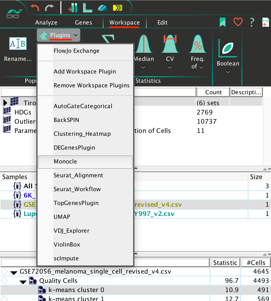
Note: R will not run if the file path leading to your GeqZip workspace contains any space characters. Make sure to remove the spaces from your GeqZip file path before attempting to run plugins which rely on R.
12.3 Developers
We encourage researchers utilizing R packages, or designing their own algorithms to publish plugins for FlowJo, in order to share their important work with the world. To get these power-users started, we offer couple of resources for developers:
- Developer Guide: legacy.gitbook.com/book/flowjollc/flowjo-plugin-developers-guide/details
- Support: techsupport@flowjo.com
12.4 Highlights
Plugins for SeqGeq that get our blood pumping include (but are NOT limited to):
The Seurat pipeline plugin, which utilizes open source work done by researchers at the Satija Lab, NYU. This powerful analysis tool does a whole set of machine learning steps from a single dialog including: some quality control filtering, dimensionality reduction, KNN unbiased clustering, and differential expression analysis of those clusters.
This plugin often makes for a great first start when analyzing heterogeneous data-sets:

The Monocle plugin for pseudotime prediction, developed by the Cole Trapnell Lab. This algorithm attempts to predict biological pseudotime by investigating hypothetical trajectories leading to differentiation and terminal states. We’ve found this tool is particularly useful for investigating subsets within relatively homogeneous data, such as subpopulations of interest, allowing researchers to get the most in terms of depth from their analyses:

13. Resources
We provide a host of different channels for researchers who want to learn more about analyses in bioinformatics and single-cell research.
13.1 Educational
- FlowJo University: www.flowjo.com/learn/flowjo-university/seqgeq
- The Daily Dongle: flowjo.typepad.com/the_daily_dongle/
- The Cell Sort: www.flowjo.com/blog
- FlowJo Webinars: www.flowjo.com/learn/webinars
13.2 Research Tools
- Sanger Institute: www.sanger.ac.uk/science/programmes/archive-page-computational-genomics
- NYU Genome Center: www.nygenome.org/
- The Broad: www.broadinstitute.org
- Enrichr: amp.pharm.mssm.edu/Enrichr/
- Genomic Cytometry: genomiccytometery.com
13.3 Bioinformatics Platforms
- SeqGeq Trial: flowjo.com/solutions/seqgeq/free-trial
- Download SeqGeq: flowjo.com/solutions/seqgeq/downloads
- Download FlowJo: flowjo.com/solutions/flowjo/downloads
- Get a Quote: info.flowjo.com/flowjo-quotation-request-and-pricing
- The FlowJo Exchange (for Plugins): exchange.flowjo.com
13.4 Help
- Tech Support: seqgeq@flowjo.com
- Sales and Licensing: office@flowjo.com
- Phone: 800.366.6045